chapter 2: visualizing Data with Graphs
이 장에서는 다양한 데이터를 mathplotlib를 통해 표현하는 방법을 배우도록 하겠다.
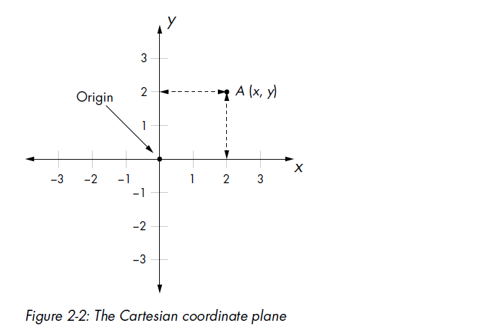
2.1 Understanding the Cartesian Coordinate Plane
다음처럼 숫자가 새겨진 라인을 생각해 보자.

아래는 Cartesian coordinate plane 을 나타낸다.
Working with Lists and Tuples
그래프를 그릴때 list,tuple을 많이 사용하게 될것이다.
Iterating over a List or Tuple
>>> l = [1, 2, 3]
>>> for item in l:
print(item)

>>> l = [1, 2, 3]
>>> for index, item in enumerate(l):
print(index, item)
Creating Graphs with Matplotlib
>>> x_numbers = [1, 2, 3]
>>> y_numbers = [2, 4, 6]

>>> from pylab import plot, show
>>> plot(x_numbers, y_numbers)
[<matplotlib.lines.Line2D object at 0x7f83ac60df10>]

plot(x_numbers, y_numbers, marker='o')

plot(x_numbers, y_numbers, 'o')
Graphing the Average Annual Temperature in New York City
from pylab import plot, show

nyc_temp = [53.9, 56.3, 56.4, 53.4, 54.5, 55.8, 56.8, 55.0, 55.3, 54.0, 56.7, 56.4, 57.3]


years = range(2000, 2013)


#plot(nyc_temp, marker='o')

years = range(2000, 2013)
plot(years, nyc_temp, marker='o')

show()
Comparing the Monthly Temperature Trends of New York City
from pylab import plot,show
from pylab import legend
legend([2000, 2006, 2012])


nyc_temp_2000 = [31.3, 37.3, 47.2, 51.0, 63.5, 71.3, 72.3, 72.7, 66.0, 57.0, 45.3, 31.1]
nyc_temp_2006 = [40.9, 35.7, 43.1, 55.7, 63.1, 71.0, 77.9, 75.8, 66.6, 56.2, 51.9, 43.6]
nyc_temp_2012 = [37.3, 40.9, 50.9, 54.8, 65.1, 71.0, 78.8, 76.7, 68.8, 58.0, 43.9, 41.5]

months = range(1, 13)

#plot(months, nyc_temp_2000, months, nyc_temp_2006, months, nyc_temp_2012)

#===============================================================================
# plot(months, nyc_temp_2000)
# plot(months, nyc_temp_2006)
# plot(months, nyc_temp_2012)
#===============================================================================

plot(months, nyc_temp_2000, months, nyc_temp_2006, months, nyc_temp_2012)

show()
Customizing Graphs
Adding a Title and Labels
from pylab import plot, show, title, xlabel, ylabel, legend

months = range(1, 13)

nyc_temp_2000 = [31.3, 37.3, 47.2, 51.0, 63.5, 71.3, 72.3, 72.7, 66.0, 57.0, 45.3, 31.1]
nyc_temp_2006 = [40.9, 35.7, 43.1, 55.7, 63.1, 71.0, 77.9, 75.8, 66.6, 56.2, 51.9, 43.6]
nyc_temp_2012 = [37.3, 40.9, 50.9, 54.8, 65.1, 71.0, 78.8, 76.7, 68.8, 58.0, 43.9, 41.5]


plot(months, nyc_temp_2000, months, nyc_temp_2006, months, nyc_temp_2012)

title('Average monthly temperature in NYC')
xlabel('Month')
ylabel('Temperature')
legend([2000, 2006, 2012])

show()
Customizing the Axes
from pylab import plot, show, axis

nyc_temp = [53.9, 56.3, 56.4, 53.4, 54.5, 55.8, 56.8, 55.0, 55.3, 54.0, 56.7, 56.4, 57.3]
plot(nyc_temp, marker='o')
print(axis())
axis(ymin=0)

show()
Plotting Using pyplot
   '''
   Simple plot using pyplot
   '''
   import matplotlib.pyplot
   def create_graph():
       x_numbers = [1, 2, 3]
       y_numbers = [2, 4, 6]
       matplotlib.pyplot.plot(x_numbers, y_numbers)
       matplotlib.pyplot.show()

   if __name__ == '__main__':
       create_graph()

Saving the Plots
from pylab import plot, savefig
x = [1, 2, 3]
y = [2, 4, 6]
plot(x, y)
savefig('mygraph.png')

#savefig('C:\mygraph.png')
Plotting with Formulas
Newton’s Law of Universal Gravitation
Newton’s law of universal gravitation

'''
The relationship between gravitational force and
distance between two bodies
'''
import matplotlib.pyplot as plt
# Draw the graph
def draw_graph(x, y):
    plt.plot(x, y, marker='o')
    plt.xlabel('Distance in meters')
    plt.ylabel('Gravitational force in newtons')
    plt.title('Gravitational force and distance')
    plt.show()

def generate_F_r():
# Generate values for r
    r = range(100, 1001, 50)
# Empty list to store the calculated values of F
    F = []
# Constant, G
    G = 6.674*(10**-11)
# Two masses
    m1 = 0.5
    m2 = 1.5
# Calculate force and add it to the list, F
    for dist in r:
        force = G*(m1*m2)/(dist**2)
        F.append(force)
# Call the draw_graph function
    draw_graph(r, F)
if __name__=='__main__':
    generate_F_r()


Generating Equally Spaced Floating Point Numbers
'''
Generate equally spaced floating point
numbers between two given values
'''
def frange(start, final, increment):
    numbers = []
    while start < final:
        numbers.append(start)
        start = start + increment
        return numbers
Drawing the Trajectory
'''
Draw the trajectory of a body in projectile motion
'''
from matplotlib import pyplot as plt
import math
def draw_graph(x, y):
    plt.plot(x, y)
    plt.xlabel('x-coordinate')
    plt.ylabel('y-coordinate')
    plt.title('Projectile motion of a ball')
def frange(start, final, interval):
    numbers = []
    while start < final:
        numbers.append(start)
        start = start + interval
        return numbers
def draw_trajectory(u, theta):
    theta = math.radians(theta)
    g = 9.8
# Time of flight
    t_flight = 2*u*math.sin(theta)/g
# Find time intervals
    intervals = frange(0, t_flight, 0.001)

    # List of x and y coordinates
    x = []
    y = []
    for t in intervals:
        x.append(u*math.cos(theta)*t)
        y.append(u*math.sin(theta)*t - 0.5*g*t*t)
        draw_graph(x, y)
if __name__ == '__main__':
    try:
        u = float(input('Enter the initial velocity (m/s): '))
        theta = float(input('Enter the angle of projection (degrees): '))
    except ValueError:
        print('You entered an invalid input')
    else:
        draw_trajectory(u, theta)
        plt.show()
Comparing the Trajectory at Different Initial Velocities
'''
Draw the trajectory of a body in projectile motion
'''
from matplotlib import pyplot as plt
import math
def draw_graph(x, y):
    plt.plot(x, y)
    plt.xlabel('x-coordinate')
    plt.ylabel('y-coordinate')
    plt.title('Projectile motion of a ball')
def frange(start, final, interval):
    numbers = []
    while start < final:
        numbers.append(start)
        start = start + interval
        return numbers
def draw_trajectory(u, theta):
    theta = math.radians(theta)
    g = 9.8
# Time of flight
    t_flight = 2*u*math.sin(theta)/g
# Find time intervals
    intervals = frange(0, t_flight, 0.001)

    # List of x and y coordinates
    x = []
    y = []
    for t in intervals:
        x.append(u*math.cos(theta)*t)
        y.append(u*math.sin(theta)*t - 0.5*g*t*t)
        draw_graph(x, y)
if __name__ == '__main__':
    # List of three different initial velocities
    u_list = [20, 40, 60]
    theta = 45
    for u in u_list:
        draw_trajectory(u, theta)
# Add a legend and show the graph
    plt.legend(['20', '40', '60'])
    plt.show()